OECD Meat Consumption Data Analysis 6 - POULTRY Consumption is positively correlated with GDP

Photo by corina ardeleanu on Unsplash 

www.crosshyou.info

This post is following of above post.

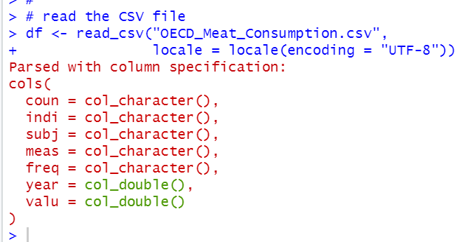
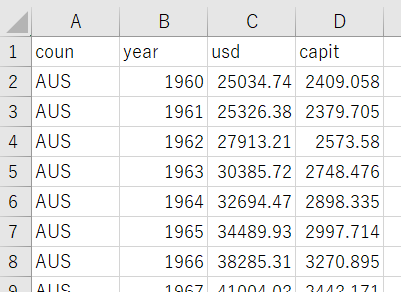
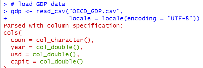
I have GDP data like below CSV file.

So, let's combine this GDP data and Meat Consumption data.

Next, I use inner_join() function to combine df2 dataframe and gdp dataframe.

Let's see the result.

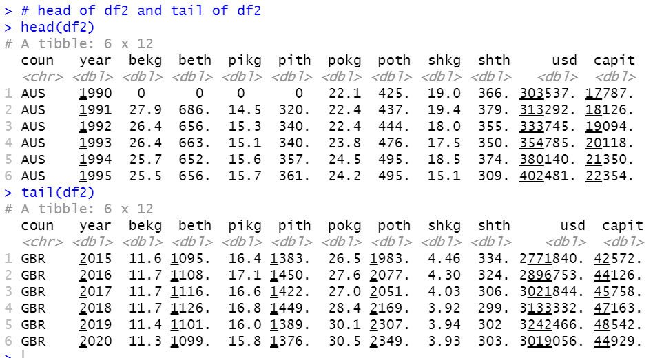
usd is gross GDP value, capit is per capita GDP.

summary if df2

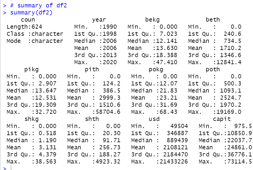
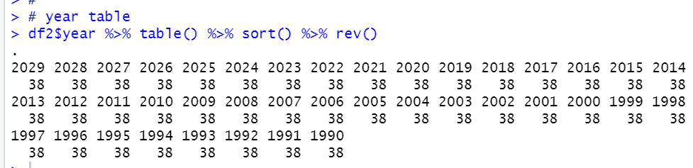
We see year range is changed. 1990 ~ 2020.

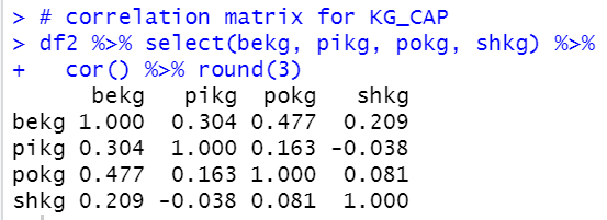
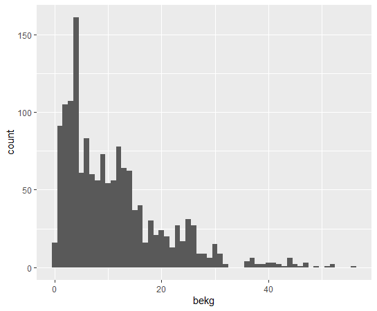
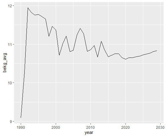
Now, let's see capit and 4 KG_CAP data.

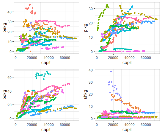
I see shkg is not so much correlated with capit.

Let's see correlation with capit and 4 KG_CAPs by country.

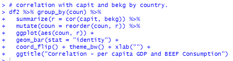
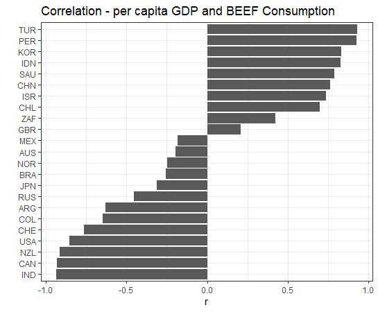
We see some countries have negative correlations and some contries have positive correlations.

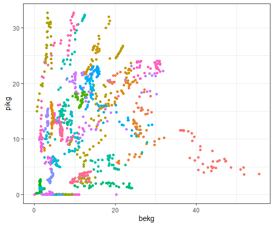
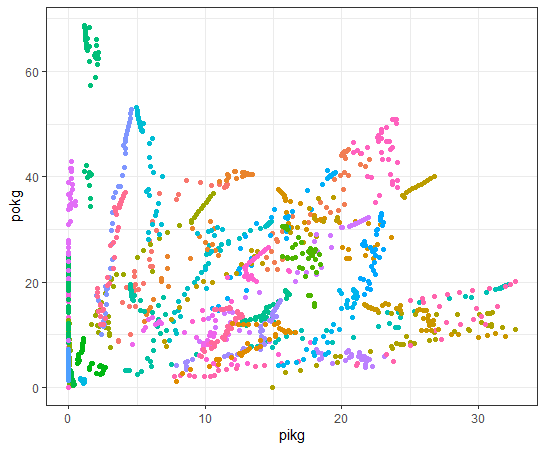
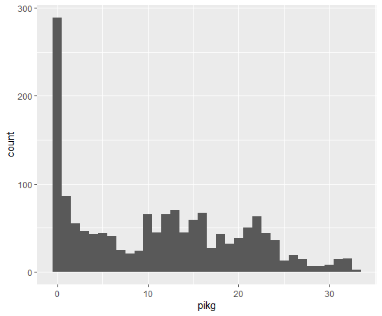
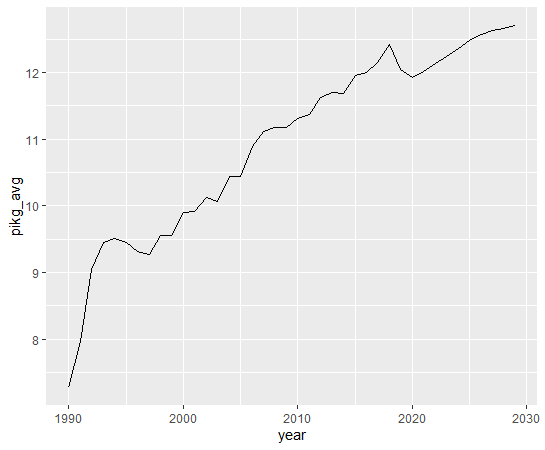
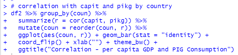
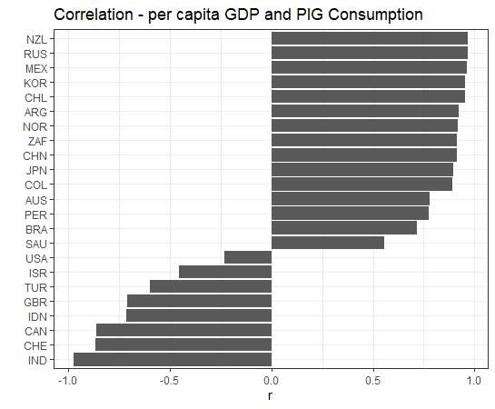
How about pikg: PIG KG_CAP?

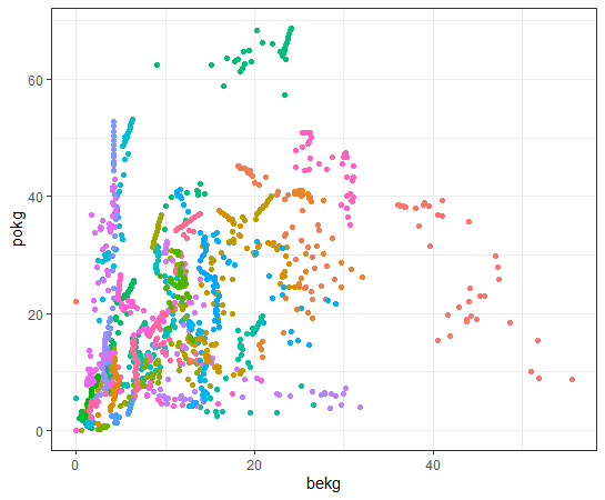
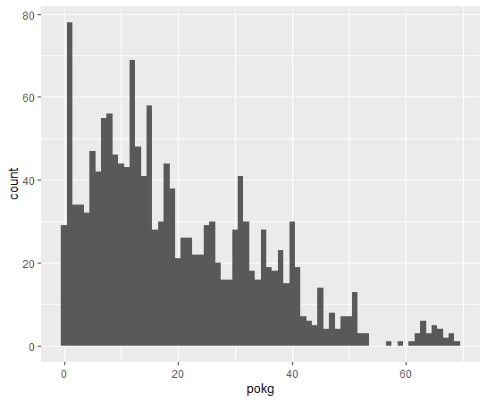
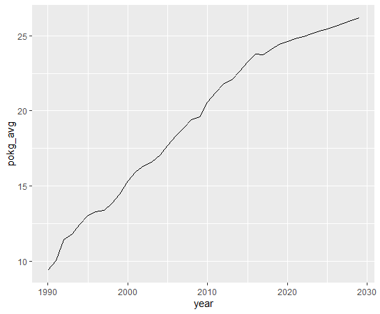
How about POULTRY?

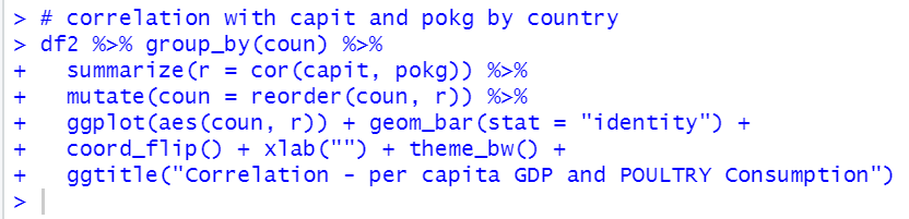
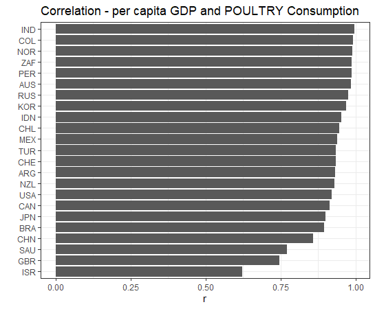
All countires have positive correlations with POULTRY.

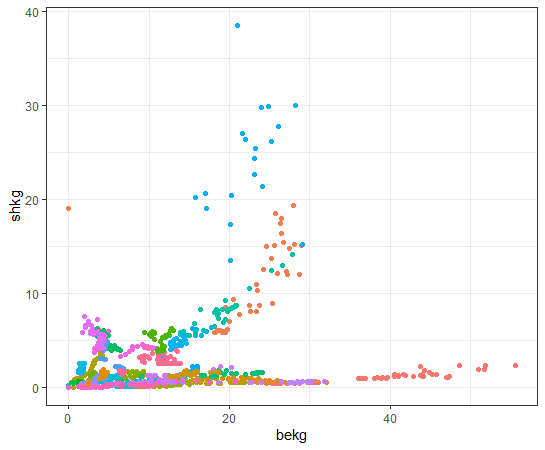
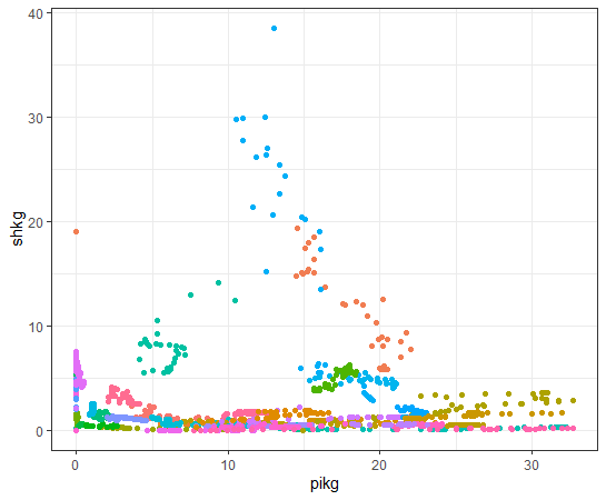
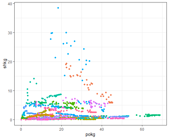
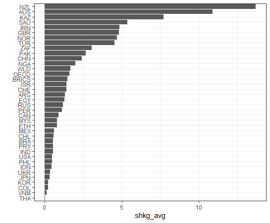
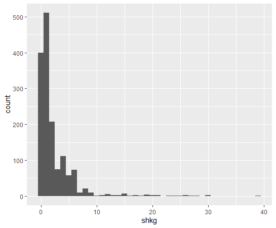
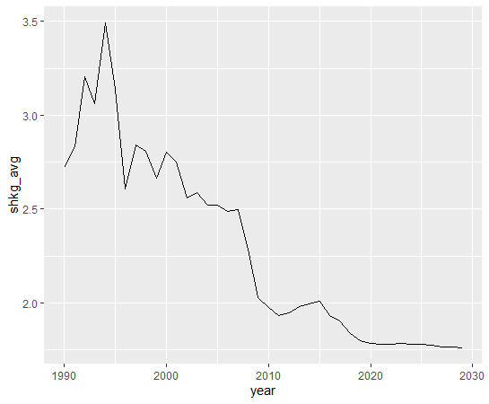
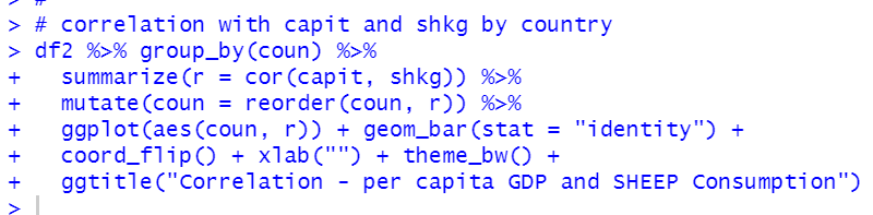
Last, how about shkg?

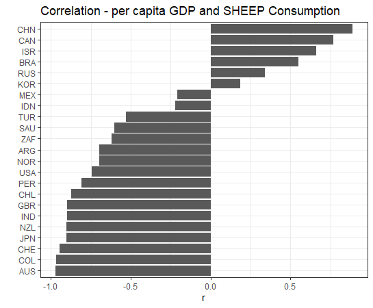
We see some countries have negative correlation while some countries have positive correlations.

per capita POULTRY Consumption and per capita GDP are positively correlated in all countries.

That's it. Thank you!

Next post is

www.crosshyou.info

To read the 1st post,

www.crosshyou.info

OECD Meat Consumption Data Analysis 5 - scatter plot using R ggplot2::geom_point()

Photo by Casey Horner on Unsplash 

www.crosshyou.info

This post is following of above post.
In this post, let's draw scatter plots using R ggplot2::geom_point.
First of all, let's see correlations about 4 KG_CAPs.

bekg: BEEF KG_CAP and pokg: POULTRY KG_CAP are the most strongly correlated pair.

pikg: PIG KG_CAP and shkg: SHEEP KG_CAP are the least weakly correlated pair.

Then, let's draw scatter plots. 
First, bekg: BEEF KG_CAP and pikg: PIG KG_CAP

We see some countries seems have negative correlation.

Let's see bekg and pokg: POULTRY KG_CAP

How about bekg and shkg: SHEEP KG_CAP?

Many countries have relatively low value for shkg compared to bekg.

pikg and pokg

pikg and shkg

Lastly, pokg and shkg

Now, we have 6 scatter plot objects, p1 ~ p6.
Let's show it at once. we use gridExtra::grid.arrange() function.

That's it. Thank you!

Next post is

www.crosshyou.info

To read the 1st post,

www.crosshyou.info

OECD Meat Consumption Data Analysis 4 - USA is the most meat consumption country.

Photo by Claiton Conto on Unsplash 

www.crosshyou.info

This post is following of above post.
Let's see KG_CAP data as country average.

Firstly, bekg: BEEK KG_CAP

ARG is the highest beef consumption country. IND is the lowest.

How about pikg: PIG KG_CAP?

TUR, PAK and IRN does not eat PIG.

poke: POULTRY KG_CAP

ISR is the highest consumption country for POULTRY.

Next, shkg: SHEEP KG_CAP

All right, let's see total(BEEF + PIG + POULTRY + SHEEP) KG_CAP.

USA is the most Meat Consumption country.

That's it. thank you!

Next post is

www.crosshyou.info

To see the 1st post,

www.crosshyou.info

OECD Meat Consumption Data Analysis 3 - PIG and POULTRY are on up trend while BEEF and SHEEP are on down trend.

Photo by Nathan Anderson on Unsplash 

www.crosshyou.info

This post is following of above post.

Let's see coun: country.

We see all country have 40 observations.

Let's see year

We see all year have 38 observations.
So, df2 data frame is 40 coun * 38 year = 1520 observations.

Let's see histograms for KG_CAP data.

First, bekg: BEEF KG_CAP

pikg: PIG KG_CAP

pokg: POULTRY KG_CAP

shkg: SHEEP KG_CAP

We see POULTRY is most normaly spread.

Next, let's see time trend.

We will see average KG_CAP by year.

First, bekg: BEEF KG_CAP

pikg: PIG KG_CAP time trend

pokg: POULTRY KG_CAP time trend

shkg: SHHEP KG_CAP time trend

We see BEEF and SHEEP are on down trend and PIG and POULTRY are on up trend.
That's it. Thank you!

Next post is

www.crosshyou.info

To read the 1st post,

www.crosshyou.info

OECD Meat Consumption Data Analysis 2 - PIG is the most popular meat.

Photo by boris misevic on Unsplash 

www.crosshyou.info

This post is following above post.
Now, we now there are 4 sunjects and 2 measures.

4 subjects are BEEG, PIG, POULTRY and SHEEP.

2 measures are KG_CAP and THND_TONNE.
So, we have 8 combinations for them.

Let's make dataframes for each combination.

BEEF and KG_CAP

BEEF and THND_TONNE

PIG and KG_CAP

PIG and THND_TONNE

POULTRY and KG_CAP

POULTRY and THND_TONNE

SHEEP and KG_CAP

SHEEP and THND_TONNE

Then, I use inner_join() function to merge those 8 dataframes into one dataframe.

All right, let's use summary() function to see summary statistics.

variable mame ~~ kg means KG_CAP, it is per capita consumption and ~~ th means THSN_TONNE, it is total consumption.

Let's see bekg: BEEF KG_CAP, pikg: PIG KG_CAP, pokg: POULTRY KG_CAP and shkg: SHEEP KG_CAP.

pikg has the largest mean, so we find PIG is the most widely eaten meat. 

That's it. Thank you!

Next post is.

www.crosshyou.info

To read the 1st post,

www.crosshyou.info

OECD Meat Consumption Data Analysis 1 - Using R to read CSV data with read_csv() function.

Photo by Wolfgang Hasselmann on Unsplash 

Hello! This post, I will anaysis OECD Meat Consumption data using R.

I got a CSV file like below from OECD web site(Agricultural output - Meat consumption - OECD Data)

Firstly, I load tidyverse package, which is very useful package for data science.

Let's read the CSV file with read_csv() function.

Let's see each variables.

coun is country name.

We see all countries have 320 observations.

indi is indicator.

indi ha sonly one value, MEATCONSUMP, so we need not keep this variable in our dataframe.

subj means subject.

subj has 4 kinds of value, SHEEP, POULTRY, PIG and BEEF. Each subj has 3040 observations. I convert subj to factor class.

meas is measure.

meas has two kind of value, THND_TINNE and KG_CAP. I convert meas to factor class.

feq is frequency.

freq ha only one value, A, I will remove freq from my data frame.

year is year.

The oldest year is 1990, the newest year is 2029! Maybe this data frame is including estimated data.

valu is meat consumption value.

Median is 24.77 and Mean is 2291.58, so I see there is skewd data.

Let's see summary of my data frame.

That's it!
Thank you!

Next post is

www.crosshyou.info

都道府県別の仕事の平均時間のデータ分析７ - 女性の仕事の平均時間は、１人当たり県民所得が高くなると短くなる。

Photo by Xavier von Erlach on Unsplash 

www.crosshyou.info

の続きです。

こんどは、male_m: 男性の仕事の平均時間(分)を回帰分析してみます。

P-valueが0.703ということなので、有意なモデルではないです。

step関数でモデルを単純化してみます。

female_m: 女性の仕事の平均時間(分)だけがかろうじて残りました。ただ、female_mの係数のp値は0.112ですから10%水準でも有意ではありません。

つまり、男性の仕事の平均時間は１人当たり県民所得や300人以上の事業所に勤める従業者割合や東日本、西日本による違いや、大きな都府県などそのような要因とは関係ないということですね。

female_m: 女性の仕事の平均時間(分)を回帰分析してみます。

こちらのモデルのp値は2.937e-05なので有意なモデルです。

big6とnoseaは5%以下の水準で有意ですし、inc, male, female, male_mは10%以下の水準で有意です。

coef()関数とround()関数で係数をわかりやすく表示します。

big6を見ると、東京都、神奈川県、千葉県、埼玉県、愛知県、大阪府の女性は他の条件が同じならば35分ほど仕事の平均時間が短いことを表します。

noseaを見ると、海なし県は他の条件が同じならば11分ほど仕事の平均時間が短いことを表します。

incを見ると、所得が1千円増えると他の条件が同じならば、0.01643分、仕事の平均時間が短かくなります。100万円の増加で16分短くなります。incの最小値は2002, つまり200万円、最大値は4525、つまり423万円ですですから30分強の違いが最低の所得水準と最高の所得水準で発生します。

今回は以上です。

男性の仕事の平均時間は、他の要因には影響されないですが、

女性の仕事の平均時間は、外部要因に影響されていることがわかりました。

今回は以上です。

はじめから読むには

www.crosshyou.info

です。