
Photo by Masako Ishida on Unsplash
This post is following of the above post.
Which chountry has many observations?
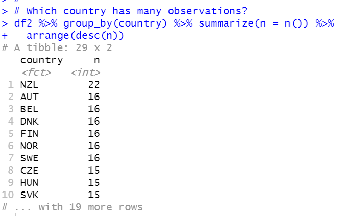
NZL has 22 observations.
AUT, BEL, DNK, FIN, NOR and SWE have 16 observations.
Let's see NZL data.
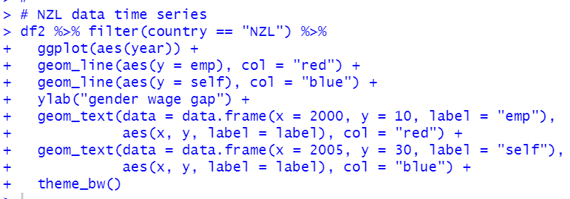
We see emplyment gender wage gap is less than selfemploy gender wage gap.
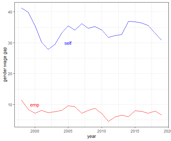
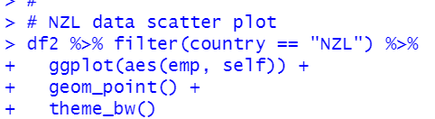
Let's see scatter plot.
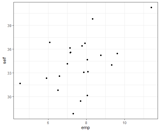
There seems positive correlation.
Let's check it.
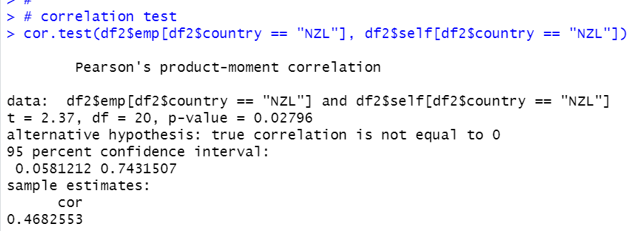
p-value is 0.02796 and correlation is 0.4682.
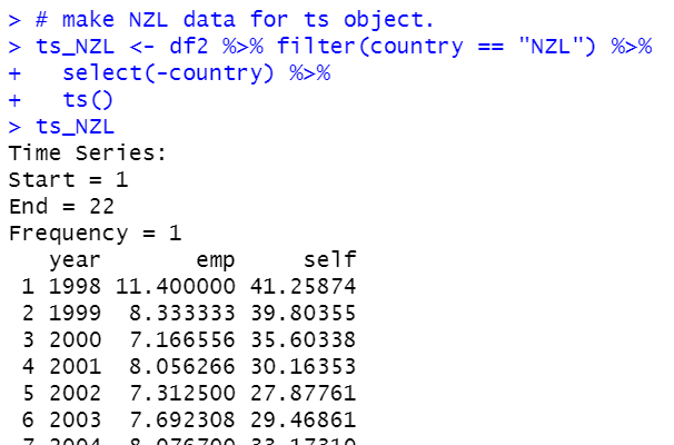
I make NZL only time series data object.
Then, let's see linear regression of static model.
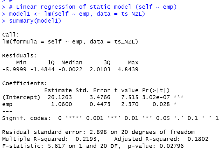
p-value is 0.02796. So this model is statistically significant under 5% confidence level.
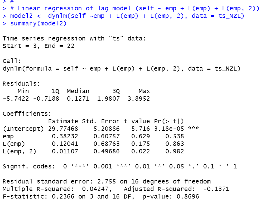
Then, let's see linear regression of model with lag.
Firstly, load dynlm package.
Then, I ise dynlm() function.
Then, let's test H0: all 'emp' coefficients are = 0.
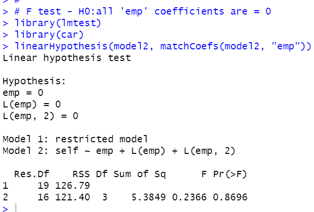
p-value is 0.8696, so we faile to reject H0.
Next, let's add trend factor.
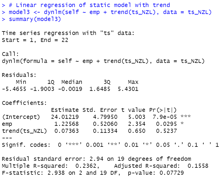
After adding trend factor to static model, emp is still significant.
Let's make a result table with stargazer package.
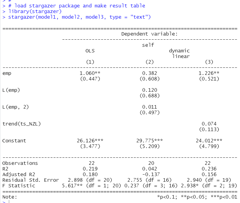
That's it. Thank you!
Next post is
To see the 1st post..