OECD Material productivity data analysis 4 - Using R for Time-Series Data analysis, static model and finite distributed lag model

Photo by mostafa meraji on Unsplash 

www.crosshyou.info

This post follow abovr post.

In the previous post, I did cross section data analysis. In this post, I do time-series data analysis.

First, let's check how many LOCATION have most data.

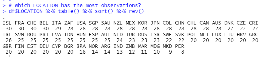
ISL, FRA, CHE and BEL have 30 observations. So I will use those locations for time-series data analysis.

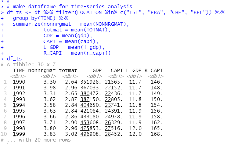
I make dataframe for time seriea analysis.

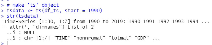
Then, I use ts() function to convert it to ts object.

It is easy to make plots with ts object.

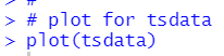
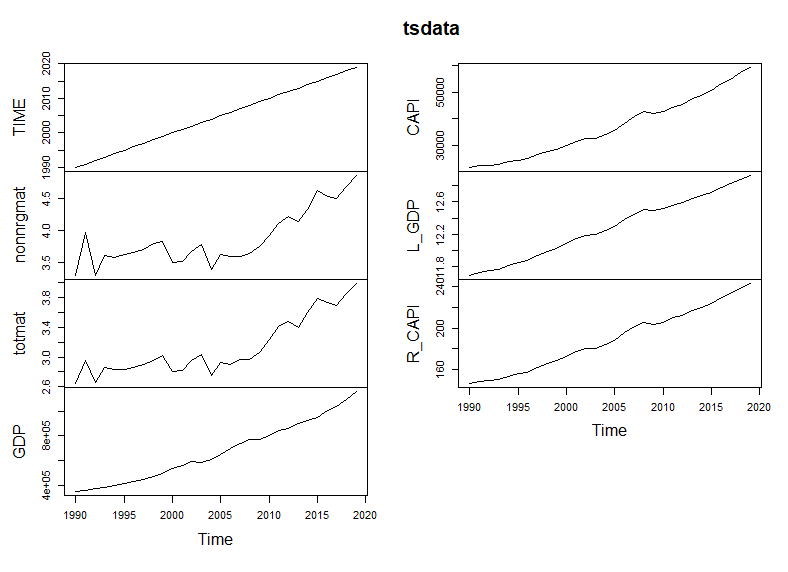
using plot() function with ts object shows line charts for each variables at onece.

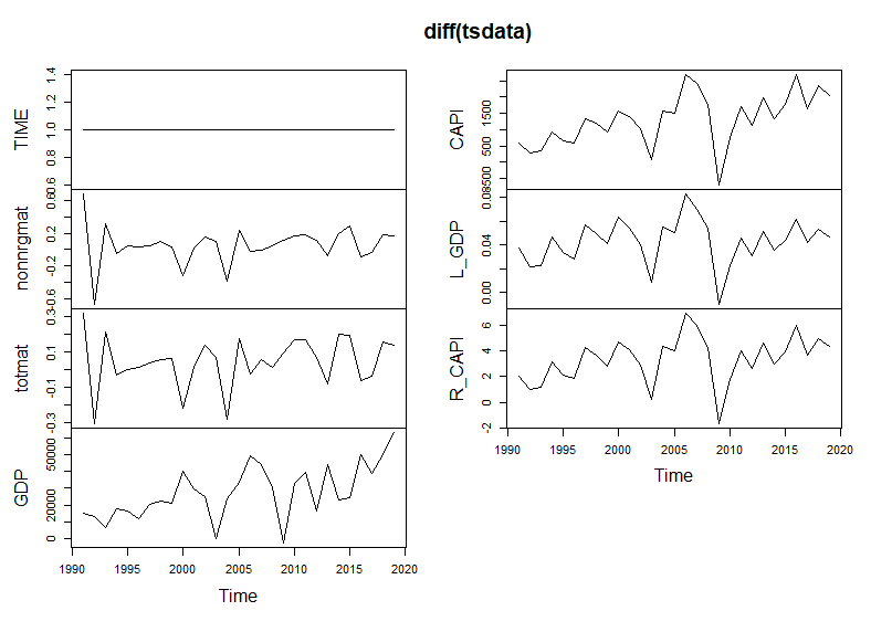
We can use diff() function to get difference.

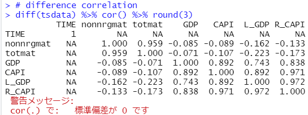
let's see correlations with cor() function.

They are strongly correlated each other.

How about difference correlation?

Then, I do time-series regression. I refer to following books.

Using R for Introductory Econometrics

Introductory Econometrics: A Modern Approach

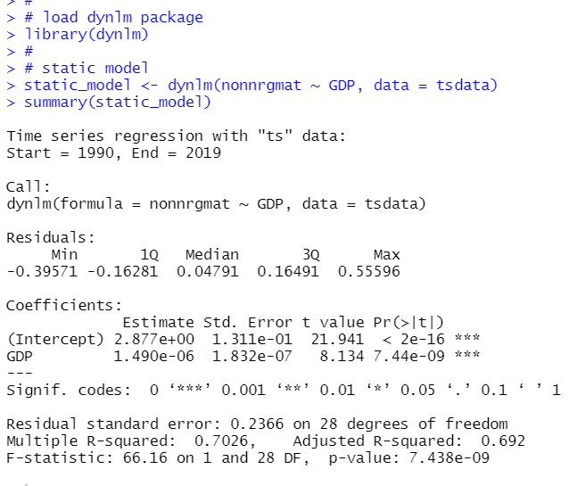
Firstly, I examine static time series models.

nonnrgmat = b0 + b1*gdp + u

Before making regression analysis, let's make a scatter plot.

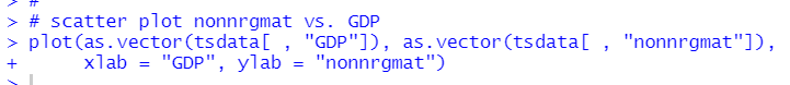
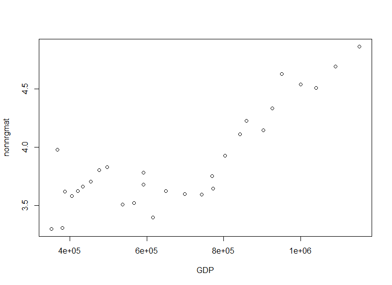
to do time-series data regression, I use dynlm package's dynlm() function.

Since nonnrgmat and GDP are too different scale, I transform GDP to GDP/1000000.

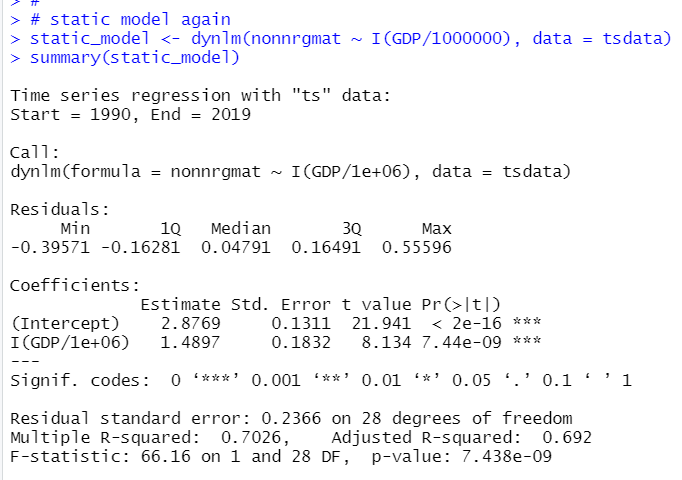
So, 1 GDP/1e+06(1 million GDP) change makes 1.4897 nonnrgmat change.

Next, I make Finite Distributed Lag model.

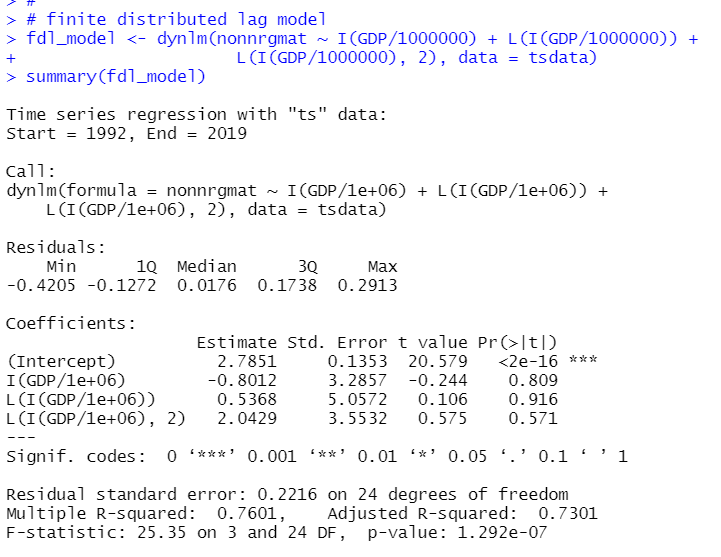
All three explanatory variables are not significant on individual base, but I assume they are jointly significant. Let's checl with linearHypothesis() function.

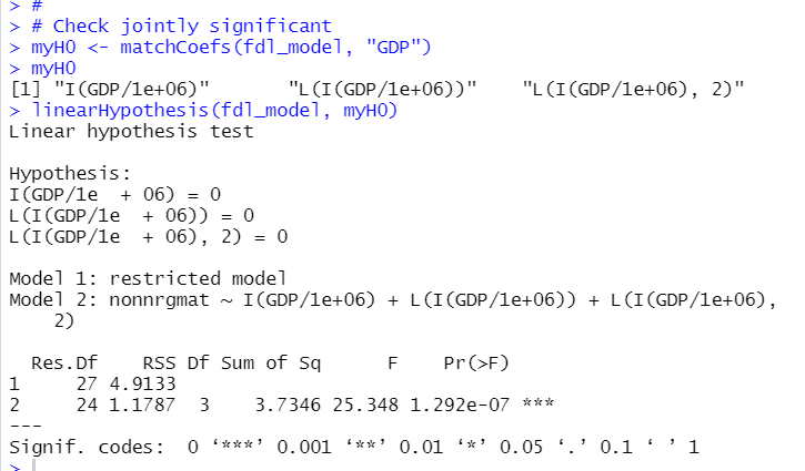
p-value is almost 0. So, I confirm that the three explanatory variables are jointly significant.
It's long run propency is -0.8012 + 0.5368 + 2.0429 = 1.7785.

That's it. Thank you!

The next post is

www.crosshyou.info

To see the first post,

www.crosshyou.info