
UnsplashのS. Tsuchiyaが撮影した写真
This post is following of the above post.
In the above post, I made a data frame to work with.
Let's check each variable names and it's explanations.
BUPSRY: Below upper secondary, in percentage
TRY: Tertiary, in percentage
UPPSRY: Upper secondary, in percentage
TRY_MEN: Tertiary men, in percentage
TRY_WOMEN: Tertiary women, in percentage
UPPSRY_MEN: Upper secondary men, in percentage
UPPSRY_WOMEN: Upper secondary women, in percentage
BUPSRY + TRY + UPPSRY = 100
MLN_USD: GDP, in million USD
USD_CAP: per capita GDP, in USD
Since I would like to see relationships between tertiary education level and GDP, I will focus TRY, TRY_MEN, TRY_WOMEN, USD_CAP.
Let's see those 4 variables summary statistics.

I see TRYs averages are arorund 27%, USD_CAP is 31,647 USD.
I would like to see standard deviation and CV(coefficient of variation)
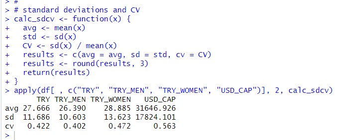
First, I make custom function to calulate mean, standard deviation and CV, then I use apply() fundtion. I see USD_CAP is the most variation.
Let's see histograms of those four variables.

I load gridExtra before making histograms.
Then, I use ggplot() + geom_histogram() function to make histogrmas and I use grid.arrange() function to display four histgrams at onece.


I see TRYs have similar shape and USD_CAP is very right skewed.
let's see log(USD_CAP) histogram.
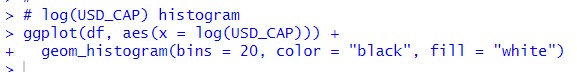

I see log(USD_CAP) is more like normal distribution, then, I make a new varibale of log(USD_CAP).
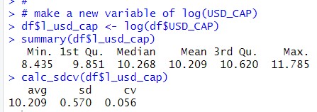
Above is summary statistics of l_usd_cap. I see CV is very small, 0.056.
That's it. Thank you!
To read from the first post,