
Generated by Bing Image Creator: last sunshine landscape of Morocco blue sky, photo
This post is following of the above post.
In the above post, I make grapsh to see variables. In this post I add gender data to those graphs so that we can see difference between male and female for each variable.

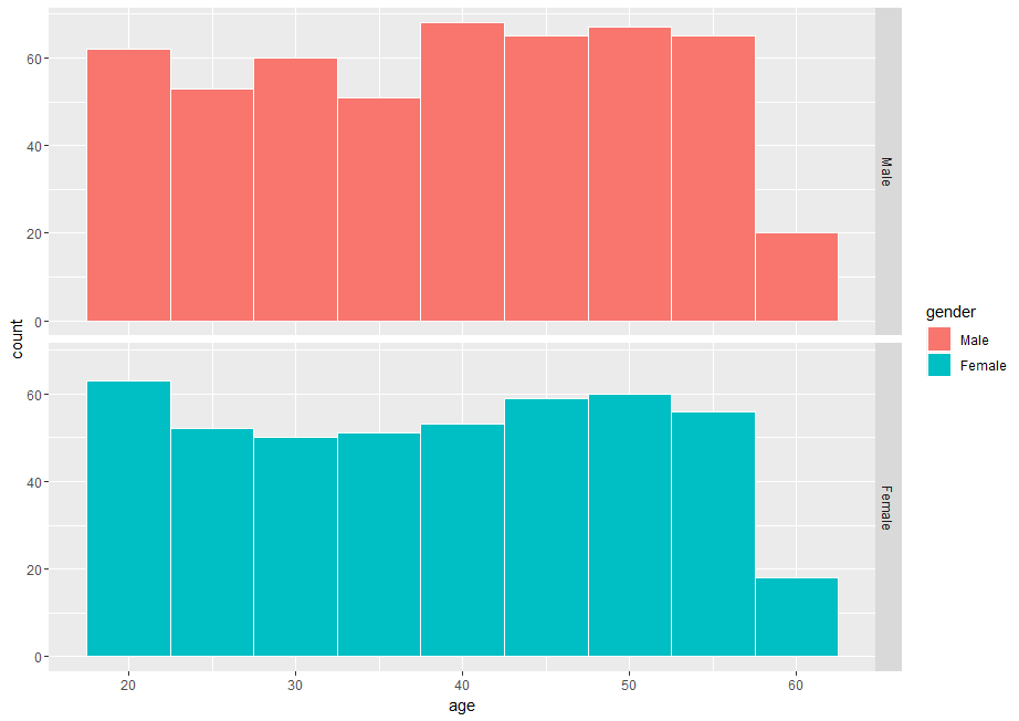
For age, there is not large difference by gender.

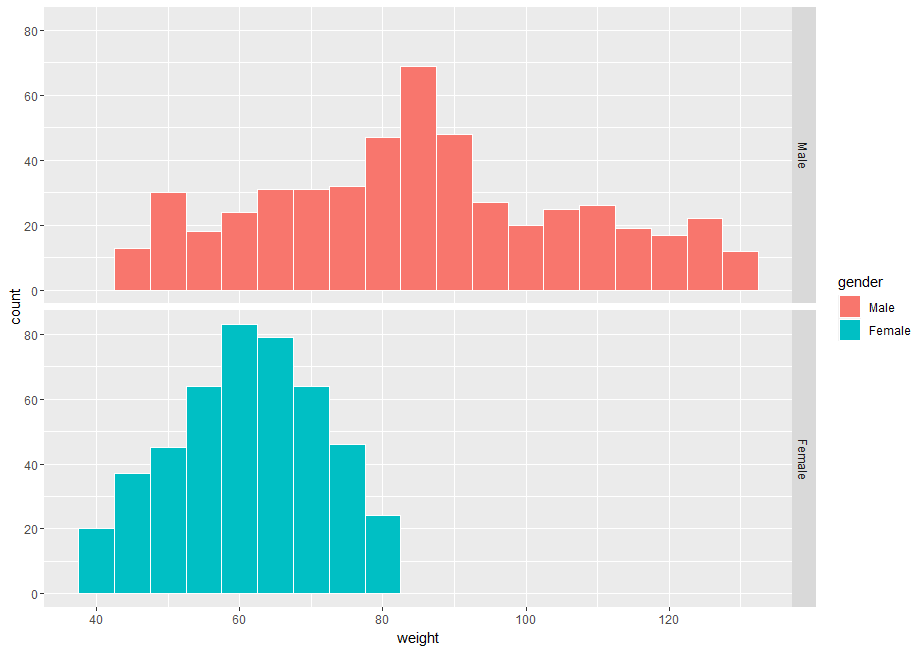
For weight, there is clearly difference by gender.

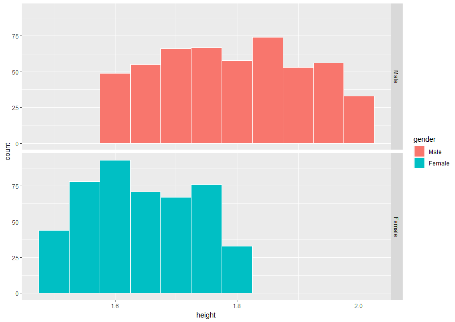
For height, there is clearly difference by gender.

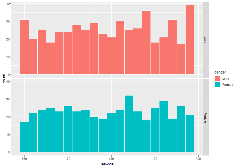
For maxbpm, there is not large difference by gender.


For avgbpm, there is not large difference by gender.

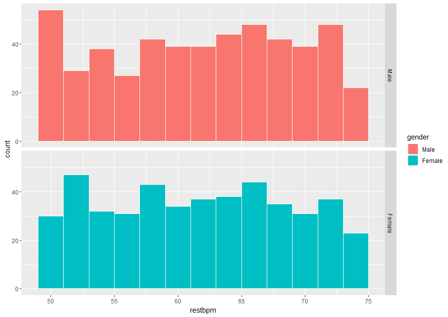
For restbpm, there is not rarge difference by gender.

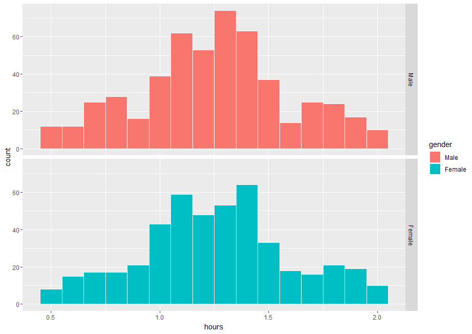
For hours, there is not large difference by gender.


For calories, there is not large difference by gender. Male has slightly large calories.


For type, there is not large difference by gender.


For fatpct, female has larger fatpct.

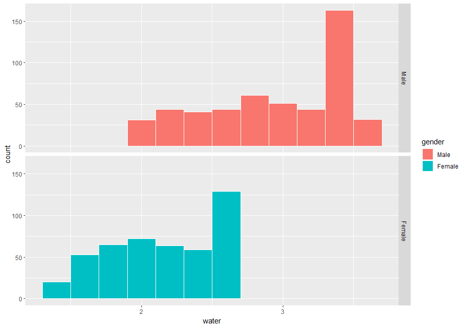
For water, male has larger water.

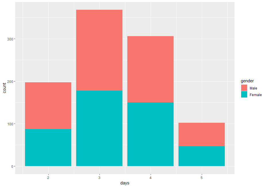
For days, there is not large difference by gender.


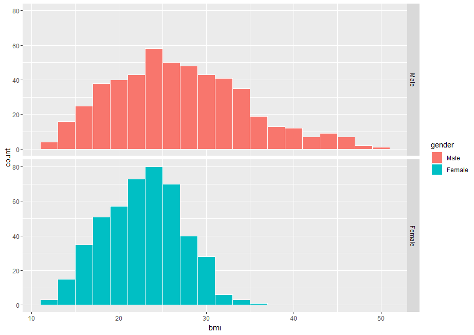
Male has lager bmi than female.
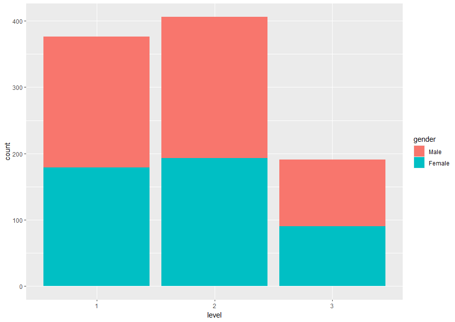
All right, I find there are two types of variables, one is differ by gender and the other does not differ by gender.
Differ by gender: weight, height, fatpct, water and bmi.
Not differ by gender: age, maxbpm, avgbpm, restbpm, hours, calories, type, days and level.
That's it. Thank you!
Next post is
To read from the first post,
This post is using below code
#
# gender and age
ggplot(gym_raw, aes(x = age, group = gender, fill = gender)) +
geom_histogram(binwidth = 5, color = "white") +
facet_grid(gender ~ .)
#
# gender and weight
ggplot(gym_raw, aes(x = weight, fill = gender)) +
geom_histogram(binwidth = 5, color = "white") +
facet_grid(gender ~ .)
#
# gender and height
ggplot(gym_raw, aes(x = height, fill = gender)) +
geom_histogram(binwidth = 0.05, color = "white") +
facet_grid(gender ~ .)
#
# gender and maxbpm
ggplot(gym_raw, aes(x = maxbpm, fill = gender)) +
geom_histogram(binwidth = 2, color = "white") +
facet_grid(gender ~ .)
#
# gender and avgbpm
ggplot(gym_raw, aes(x = avgbpm, fill = gender)) +
geom_histogram(binwidth = 2, color = "white") +
facet_grid(gender ~ .)
#
# gender and restbpm
ggplot(gym_raw, aes(x = restbpm, fill = gender)) +
geom_histogram(binwidth = 2, color = "white") +
facet_grid(gender ~ .)
#
# gender and hours
ggplot(gym_raw, aes(x = hours, fill = gender)) +
geom_histogram(binwidth = 0.1, color = "white") +
facet_grid(gender ~ .)
#
# gender and calories
ggplot(gym_raw, aes(x = calories, fill = gender)) +
geom_histogram(binwidth = 100, color = "white") +
facet_grid(gender ~ .)
#
# gender and type
ggplot(gym_raw, aes(x = type, fill = gender)) +
geom_bar()
#
# gender and fatpct
ggplot(gym_raw, aes(x = fatpct, fill = gender)) +
geom_histogram(binwidth = 2, color = "white") +
facet_grid(gender ~ .)
#
# gender and water
ggplot(gym_raw, aes(x = water, fill = gender)) +
geom_histogram(binwidth = 0.2, color = "white") +
facet_grid(gender ~ .)
#
# gender and days
ggplot(gym_raw, aes(x = days, fill = gender)) +
geom_bar()
#
# gender and level
ggplot(gym_raw, aes(x = level, fill = gender)) +
geom_bar()
#
# gender and bmi
ggplot(gym_raw, aes(x = bmi, fill = gender)) +
geom_histogram(binwidth = 2, color = "white") +
facet_grid(gender ~ .)
#