
(Bing Image Creator で生成: プロンプト: Closeup of orange Pelargonium flowers, trees are in the great large grass field, photo)
の続きです。今回はツリーモデル、決定木で予測してみます。
rpart, rpart.plot パッケージの読み込みから始めます。
rpart() 関数でモデルを生成します。
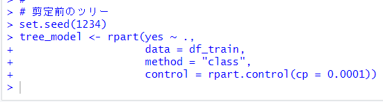
とりあえず、cp = 0.0001 にしてみました。
rpart.plot() 関数で決定木のグラフを描きます。
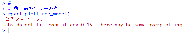
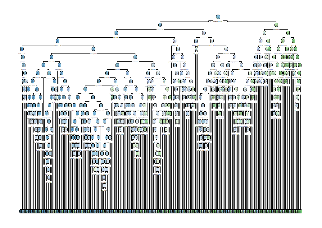
木の枝がいっぱいすぎて、何かなんだかわからない状態ですね。木というよりもブラシでしょうか・・・
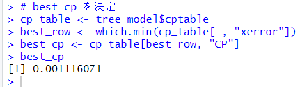
最適な cp を求めます。
このコードは何をやっているか、確認します。
はじめに作成した cp_table は
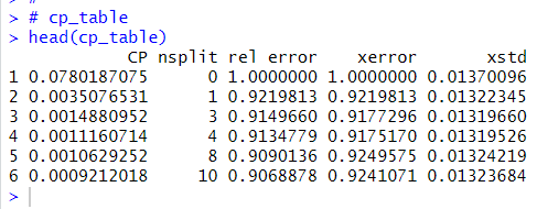
このような 表です。この表の xerror が最小の行の CP がベストの CP です。
そして、which.min() 関数で、xerror が最小の行を見つけます。
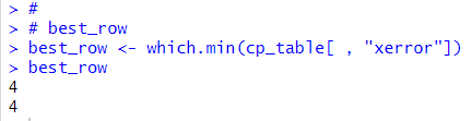
そして、4行目の CP を取り出しています。
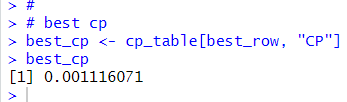
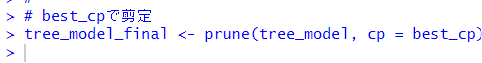
この cp = 0.00116071 でツリーモデルを剪定します。prune() 関数を使います。
剪定された木を描いてみます。
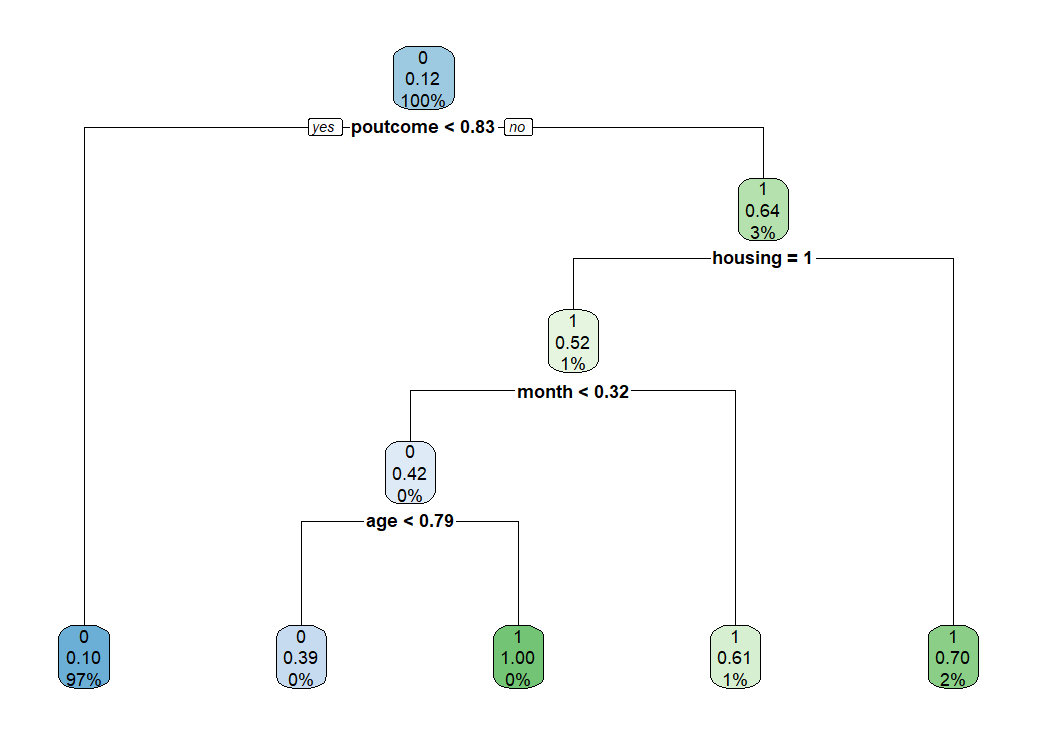
とてもスッキリとして決定木になりました。この決定木モデルで予測します。
予測結果を confusionMatrix() 関数で調べます。
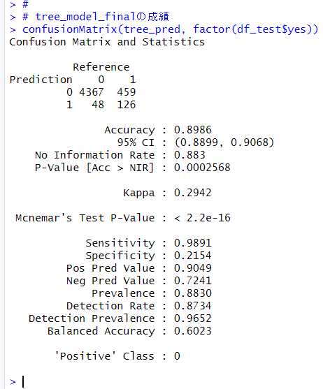
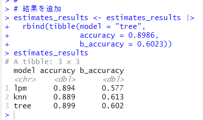
Accuracy は 0.8986, Balanced Accuracy は 0.6023 でした。
前回までの結果に追加しておきます。
今回は以上です。
次回は
です。
初めから読むには、
です。
今回のコードは以下になります。
#
# 第3のモデル: ツリーモデル
# rpart, rpart.plotパッケージの読み込み
library(rpart)
library(rpart.plot)
#
# 剪定前のツリー
set.seed(1234)
tree_model <- rpart(yes ~ .,
data = df_train,
method = "class",
control = rpart.control(cp = 0.0001))
#
# 剪定前のツリーのグラフ
rpart.plot(tree_model)
#
# best cp を決定
cp_table <- tree_model$cptable
best_row <- which.min(cp_table[ , "xerror"])
best_cp <- cp_table[best_row, "CP"]
best_cp
#
# cp_table
head(cp_table)
#
# best_row
best_row <- which.min(cp_table[ , "xerror"])
best_row
#
# best cp
best_cp <- cp_table[best_row, "CP"]
best_cp
#
# best_cpで剪定
tree_model_final <- prune(tree_model, cp = best_cp)
#
# tree_model_final をグラフに
rpart.plot(tree_model_final)
#
# tree_model_final で予測
tree_pred <- predict(tree_model_final,
df_test,
type = "class")
#
# tree_model_finalの成績
confusionMatrix(tree_pred, factor(df_test$yes))
#
# 結果を追加
estimates_results <- estimates_results |>
rbind(tibble(model = "tree",
accuracy = 0.8986,
b_accuracy = 0.6023))
estimates_results
#