
UnsplashのJean Vellaが撮影した写真
This post is following of the above post.
I made histograms in the previous post, in this post, I will make another type of graphs, boxplot.
Let's start wtih LOCATION and TRY.
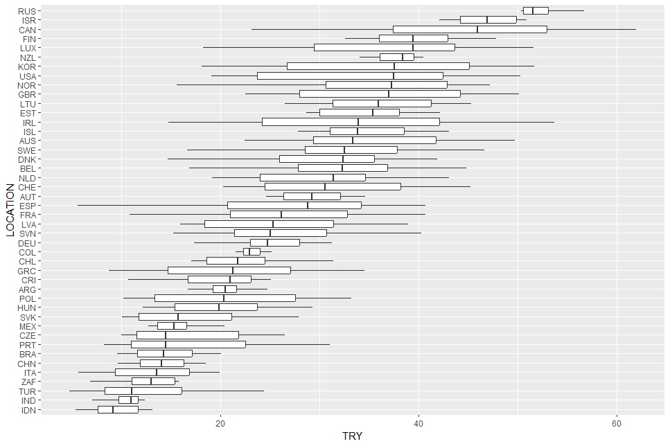
I see RUS, ISR, CAN and so on are high level locations, IDN, IND, TUR ans so on are low level locations.
Next, LOCATION and TRY_MEN
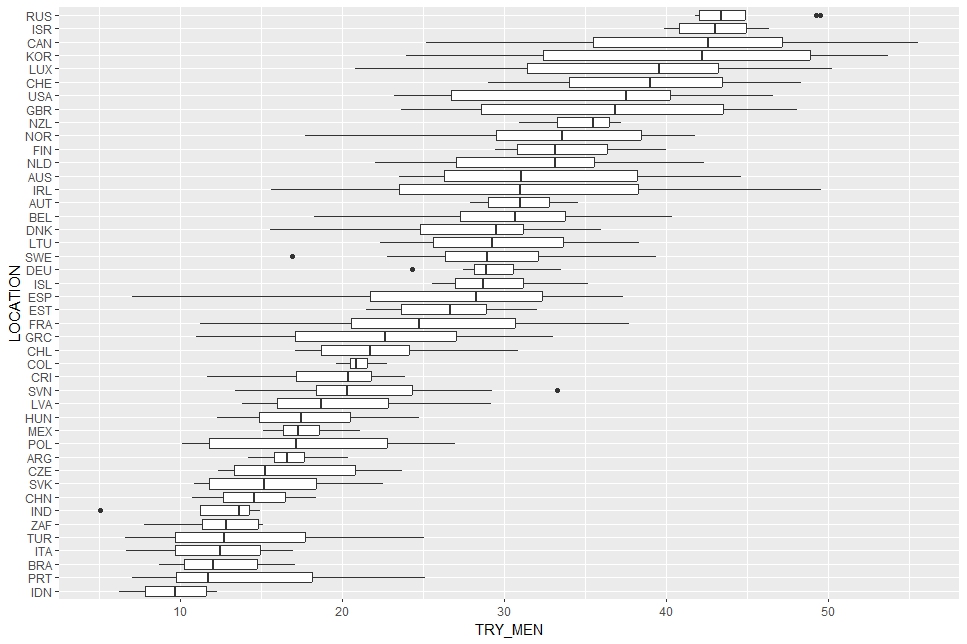
I see RUS, ISR, CAN and so on are high level, IDN, PRT, BRA and so on are low level.
Next, LOCATION and TRY_WOMEM
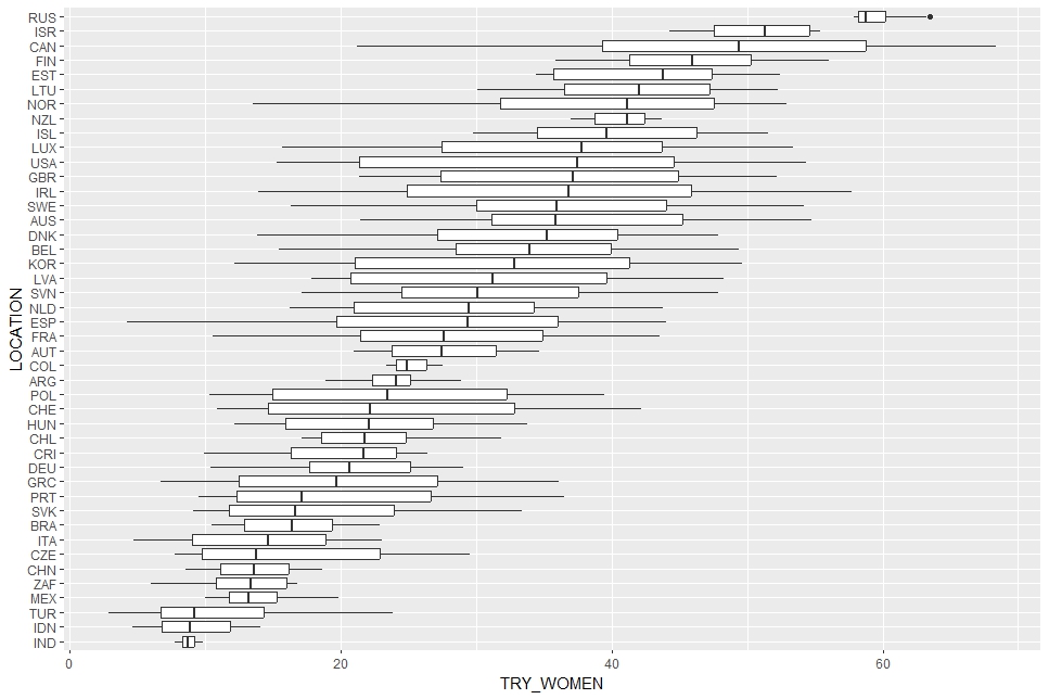
I see RUS, ISR, CAN are high level, IND, IDN, TUR are lowlevel.
Next, LOCATION and l_usd_cap
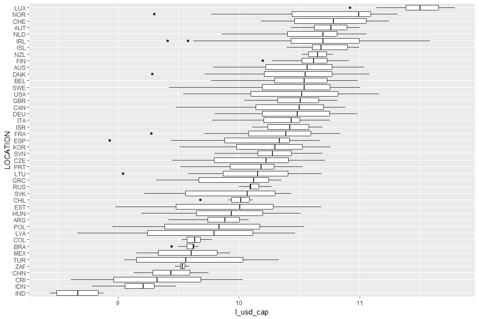
I see LUX, NOR, CHE and so on are high l_usd_cap, IND, IDN, CRI and so on are low l_usd_cap.
I observ TRY, TRY_MEN, TRY_WOMEN are very similar, so I will make another variable, the difference between TRY_MEN - TRY_WOMEN.
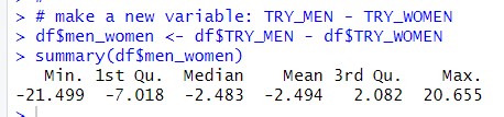
mean, median are below zero, so I find TRY_WOMEN is higher than TRY_MEN for many locations.
Let' see histogram of men_women.
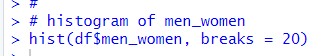
I used hist() function instead of ggplot() + geom_histogram() function because hist() is easier for just a simple histogram. men_women is distributed like normal distribution.
Then, let's see LOCATION and men_women
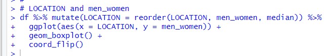
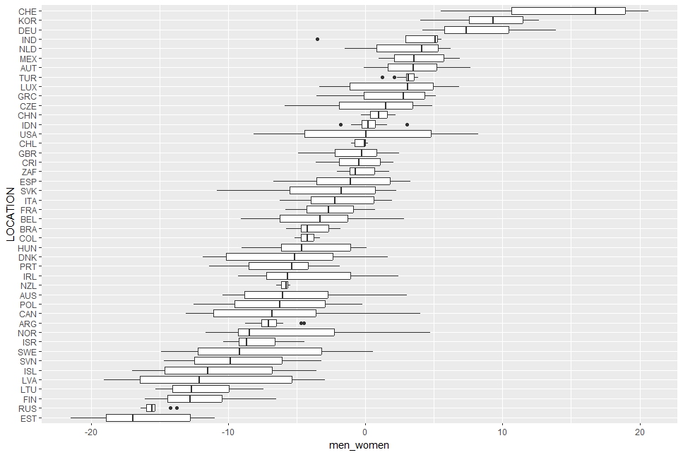
I see CHE, KOR, DEU and so on are positive men_women location while EST, RUS, FIN and so on are negative men_women location.
I get some sense of which locatiions has high level TRY and difference between men and women through above boxplots, next, let's see time trend.
I start with TIME and TRY
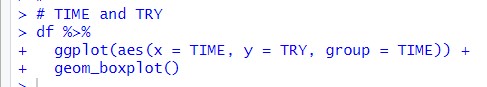
I see TRY is increaseing trend.
How about men_women?
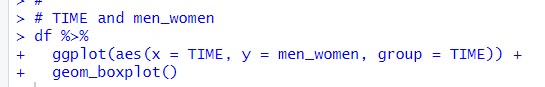
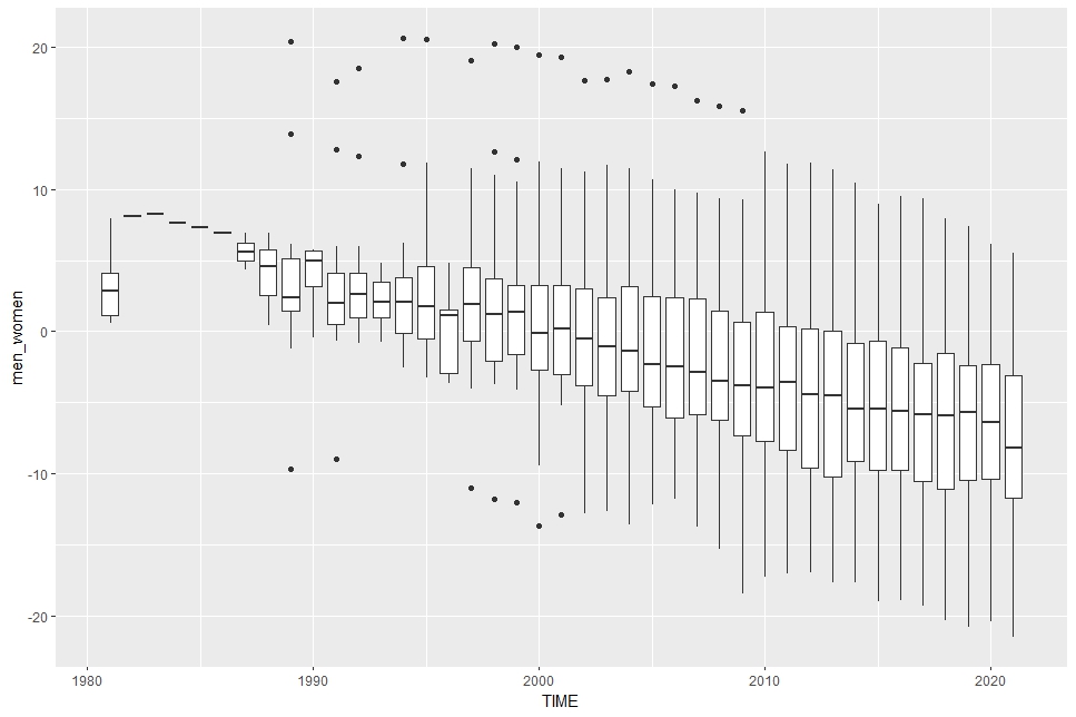
men_women is down trending, it means TRY_WOMEN is more increasing than TRY_MEN.
Next, TIME and l_usd_cap.
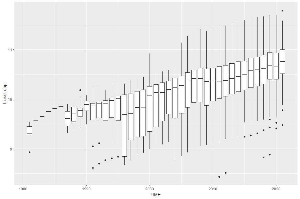
l_usd_cap is up trending.
That's it. Thank you!
Next post is
To read from the first post,