www.crosshyou.info

政府統計の総合窓口のデータや、OECDやUCIやのデータを使って、Rの練習をしています。ときどき、読書記録も載せています。

都道府県別の県議会議員の所属政党のデータの分析3 - 女性議員比率の高い都道府県、低い都道府県はどこか。東京都の女性議員比率は特別高い。


www.crosshyou.info

 の続きです。

前回の分析で全国の女性議員比率はわずか11%だとわかりました。

今回は具体的にどの都道府県が女性議員比率が高いのか、低いのかをみていきましょう。

f:id:cross_hyou:20210529203349p:plain

まずはじめにmutate関数で女性議員比率を表す変数: f_ratioを作成しました。

arrange関数で並び替えします。

f:id:cross_hyou:20210529203519p:plain

東京都は約29%で一番女性議員比率が高いことがわかります。京都府、神奈川県、滋賀県、埼玉県と続いています。

比率が低いところはどこでしょうか?

f:id:cross_hyou:20210529203659p:plain

山梨県が3%弱で一番低いです。熊本県、大分県、広島県と続いています。

hist関数でヒストグラムを作成し、女性議員比率の分布状況をみてみます。

f:id:cross_hyou:20210529203857p:plain

f:id:cross_hyou:20210529203911p:plain

右側の裾野が広い山型ですね。

boxplot関数で箱ひげ図を描いてみます。

f:id:cross_hyou:20210529204028p:plain

f:id:cross_hyou:20210529204043p:plain

上方に外れ値が一つあります。東京都ですね。

東京都の女性議員比率は他の道府県と比較すると特別高いということですね。

今回は以上です。

次回は


www.crosshyou.info

 です。

はじめからよむには、


www.crosshyou.info

 です。


都道府県別の県議会議員の所属政党のデータの分析2 - 女性議員比率は全国合計でわずか11%


www.crosshyou.info

 の続きです。

まず、どの政党の議員が多いのか少ないのか、colSums関数で各変数の合計値を見てみましょう。

f:id:cross_hyou:20210529150743p:plain

m_jimin: 男性の自民党が1237人で一番多いようですね。わかりやすいようにグラフにしてみます。

f:id:cross_hyou:20210529152621p:plain

f:id:cross_hyou:20210529152636p:plain

m_jimin: 男性の自民党、m_musho: 男性の無所属、m_shoha: 男性の諸派、m_komei: 男性の公明党と上位4つまでが男性です。

f_musho: 女性の無所属、f_kyosan: 女性の共産党、f_shoha: 女性の諸派と続きます。

議員の性別は圧倒的に男性議員が多いようです。

いろいろとデータフレームをいじくりたいので、tidyverseパッケージを読み込んでおきます。

f:id:cross_hyou:20210529153505p:plain

まずはmutate関数を使って、男性議員の数、女性議員の数の変数を作ります。

f:id:cross_hyou:20210529154411p:plain

m_total: 男性議員の数、f_total: 女性議員の数を作りました。

これを全国合計してみます。

f:id:cross_hyou:20210529154920p:plain

男性議員の合計は2340人、女性議員の合計は303人と圧倒的に男性議員が多いです。

女性議員比率は、

f:id:cross_hyou:20210529155055p:plain

11%ほどしかありません。

今回は以上です。

次回は


www.crosshyou.info

 です。

はじめから読むには、


www.crosshyou.info

 です。


都道府県別の県議会議員の所属政党のデータの分析1 - R言語のread.csv関数でデータを読み込む。

今回は都道府県別の県議会議員の所属政党のデータの分析をしてみようと思います。

政府統計の総合窓口(www.e-stat.go.jp)からデータをダウンロードしました。

f:id:cross_hyou:20210529091821p:plain

新着となっているところをクリックしたところ、下の画像のようになります。

f:id:cross_hyou:20210529091835p:plain

所属党員別人員調(R2.12.31現在)をクリックします。

f:id:cross_hyou:20210529091848p:plain

このようなエクセルファイルをダウンロードできました。これをR言語に読み込ませやすいように、下のように加工しました。

f:id:cross_hyou:20210529091901p:plain

立憲民主党や国民民主党やれいわ新選組は議員がいなかったので削除しています。

これをR言語のread.csv関数で読み込みます。

f:id:cross_hyou:20210529092541p:plain

一番目の変数名がX.U.FEFF.というヘンな文字列がついてしまっているので修正します。

f:id:cross_hyou:20210529092738p:plain

それとNAは0なので0におきかえます。

f:id:cross_hyou:20210529093120p:plain

summary関数でNAがなくなっているかどうかを確認します。

f:id:cross_hyou:20210529093304p:plain

NAがなくなっていることは確認できました。しかし、何故かprefのlengthが54もあります。47都道府県なのにおかしいですね。みてみましょう。

f:id:cross_hyou:20210529093506p:plain

沖縄の後の空白のデータも取り込まれています。削除します。

f:id:cross_hyou:20210529093815p:plain

prefのlengthが47になりました。

各変数が何を意味するか、確認しておきます。

pref: 都道府県名

m_jimin: 男性の自民党(自由民主党)

f_jimin: 女性の自民党

m_komei: 男性の公明党

f_komei: 女性の公明党

m_ishin: 男性の維新の会(日本維新の会)

f_ishin: 女性の維新の会

m_kyosan: 男性の共産党(日本共産党)

f_kyosan: 女性の共産党

m_shamin: 男性の社民党(社会民主党)

f_shamin: 女性の社民党

m_shoha: 男性の諸派

f_shoha: 女性の諸派

m_musho: 男性の無所属

f_musho: 女性の無所属

です。

今回は以上です。

 次回は


www.crosshyou.info

 です。


OECD Threatened species data analysis 5 - Bootstrap for Cinfidence Interval

 This blog is following of

www.crosshyou.info

 In this blog, I will show you how to get confidence interval with bootstrap method.

for BIRD, 95% confidence interval is 18.1 ~ 25.3 by parametric calculation.

average ± qt(0.975, d.f.)*S.E.

f:id:cross_hyou:20210523080014p:plain

We will calculate it with bootstrap method.

1. make a vector for BIRD.

f:id:cross_hyou:20210523080449p:plain

2. decide how many times calculate average

f:id:cross_hyou:20210523080630p:plain

I set it 100,000 times.

3. make a vector to stroe averages

f:id:cross_hyou:20210523080909p:plain

4. make a function to draw random samples and calculate averages.

f:id:cross_hyou:20210523081415p:plain

let's check if the function works well.

f:id:cross_hyou:20210523081705p:plain

we see 1st, 2nd and 3rd are different value, it means the function works fine.

5. use for() function to makes averages.

f:id:cross_hyou:20210523082150p:plain

6. use quantile() to get confidence interval

f:id:cross_hyou:20210523082433p:plain

That's it.

Let's make a histogram for results and vertical lines for confidence intervals.

f:id:cross_hyou:20210523083209p:plain

f:id:cross_hyou:20210523083250p:plain

The red vertical line is average, 

the blue vertical lines are confidence interval by parametric and 

the green vertical lines are confidence interval by bootstrap.

Thank you.


To read the 1st blog,


www.crosshyou.info


OECD Threatened species data analysis 4 - making bar plot with error bars in R

This blog is following of  

www.crosshyou.info

 In this blofg, I will make barplot with error bars.

1. check n(number of overbations) of each SUBJECT

f:id:cross_hyou:20210522191516p:plain

We see BIRD has 36, MAMAL has 34 and PLANT has 35 observations.

2. calculate average pf each SUBJECT

f:id:cross_hyou:20210522191642p:plain

We see BIRD has the highest average. Plant has the lowest average.

3. caclulate variance of each SUBJECT

f:id:cross_hyou:20210522191820p:plain

We see PLANT has the largest variance and MAMMAL has the smallest variance.

4. calculate S.E., standard error. Formula is sqrt(variance/n)

f:id:cross_hyou:20210522194132p:plain

We see PLANT has the largest S.E. and MAMMAL has the smallest S.E.

5. calculate C.I., confidence interval. Formula is t(alpha, d.f.)*S.E. We calculate 95% level C.I.

f:id:cross_hyou:20210522194612p:plain

6. calculate lower level of C.I. Formula is average - C.I. 

f:id:cross_hyou:20210522194750p:plain

7. calculate upper level of C.I.. Formula is average + C.I.

f:id:cross_hyou:20210522194917p:plain

All right, we get all values to make a bar plot with error bar.
We will use barplot() and arrows().

f:id:cross_hyou:20210522195229p:plain

f:id:cross_hyou:20210522195244p:plain

NIce!. Let's make a table for above data.

f:id:cross_hyou:20210522195401p:plain

That't is. Thank you for reading.

Next blog is


www.crosshyou.info


To read the first blog,


www.crosshyou.info


OECD Threatened species data analysis 3 - ANOVA(ANalysis Of VAriance) without lm() and anova()


www.crosshyou.info

 In this brlog, let's do ANOVA(Analysis of Variance).

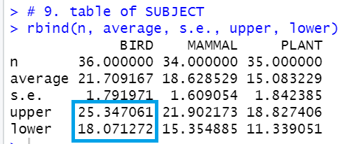
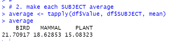
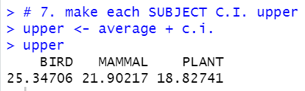
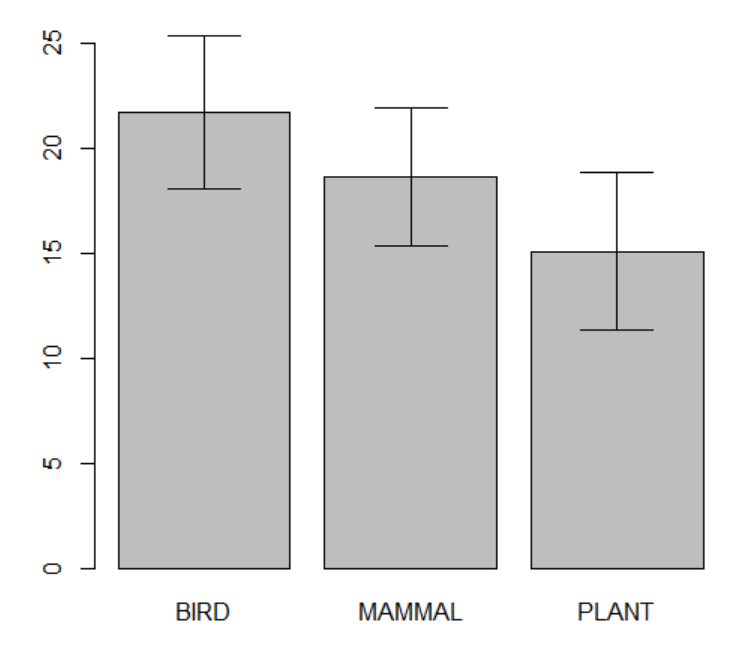
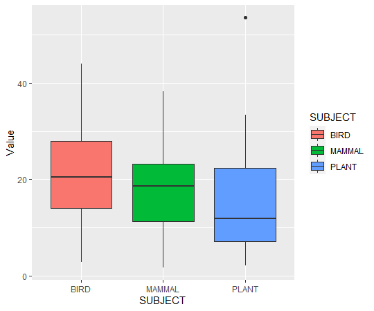
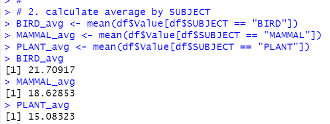
We see average Value(percentage of threatened species) are different by SUBJECT.

f:id:cross_hyou:20210522080309p:plain

BIRD has the highest Value and PLANT has the lowest.
But this difference is statistically significant?

Let's check it in R. We can use lm() function.

f:id:cross_hyou:20210522081341p:plain

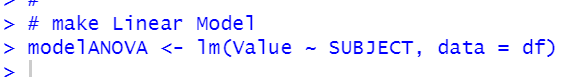
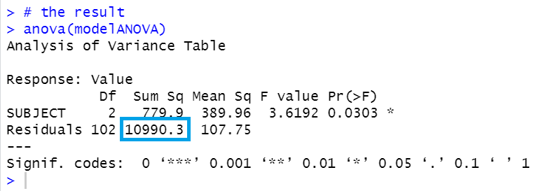
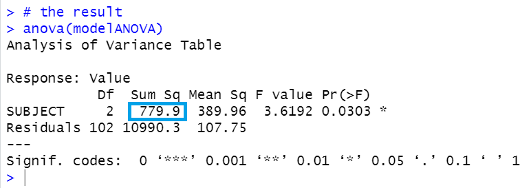
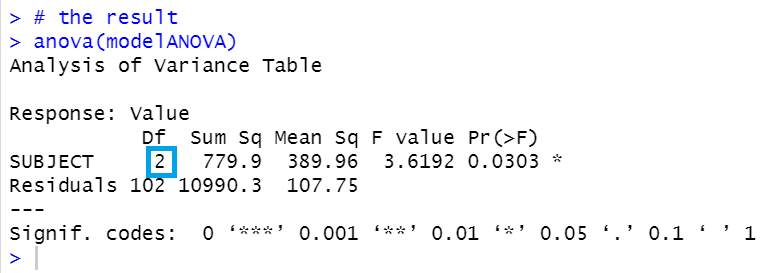
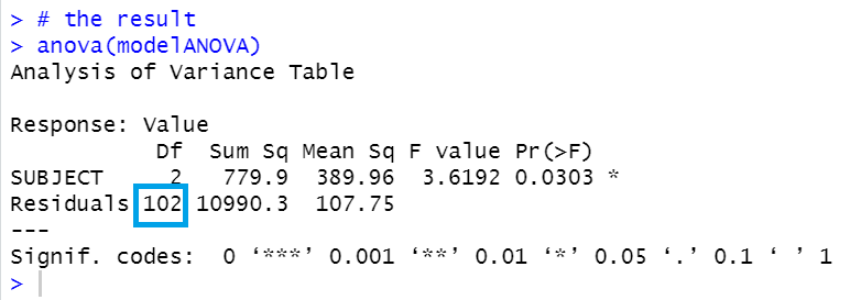
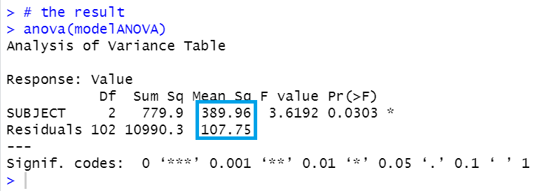
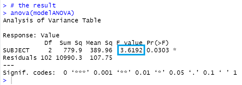
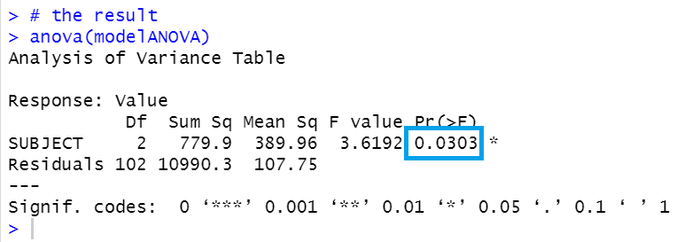
Use anova() to see the results.

f:id:cross_hyou:20210522081508p:plain

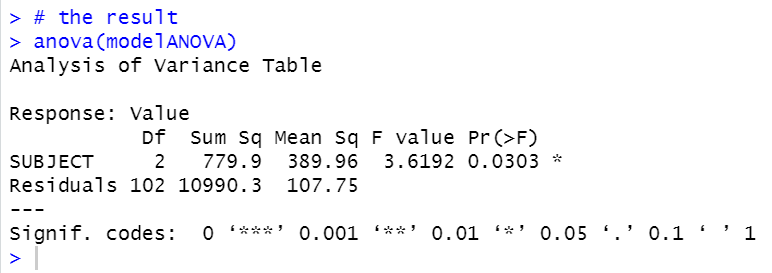
p-value is 0.0303, so it is significant at 5% significant level.

Now, let's do ANOVA without lm() and summary() function.

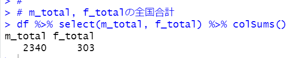
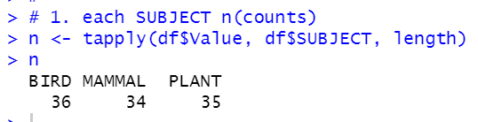
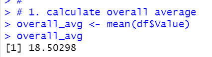
1. calculate overall average.

f:id:cross_hyou:20210522084257p:plain


f:id:cross_hyou:20210522082001p:plain

2. calculate average by SUBJECT

f:id:cross_hyou:20210522082511p:plain

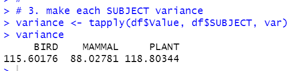
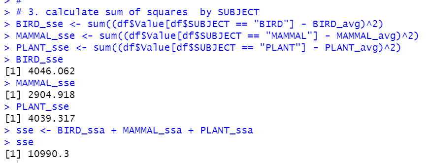
3. calculate variance by SUBJECT

f:id:cross_hyou:20210522084257p:plain

We get 10990.3

f:id:cross_hyou:20210522084538p:plain

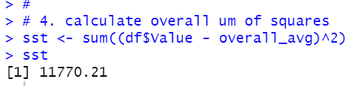
4. Calculate overall sum of squares

f:id:cross_hyou:20210522084758p:plain

5. Calculate SSE = SST - SSA
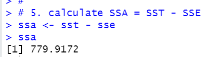
f:id:cross_hyou:20210522084936p:plain

We got 779.9

f:id:cross_hyou:20210522085042p:plain

6. calculate degree of freedom for SUBJECT
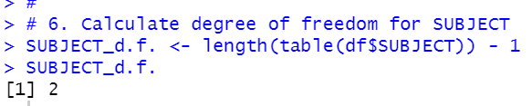
f:id:cross_hyou:20210522085328p:plain

We get 2.

f:id:cross_hyou:20210522085533p:plain

7. Calculatedegree of freedom for Residuals.
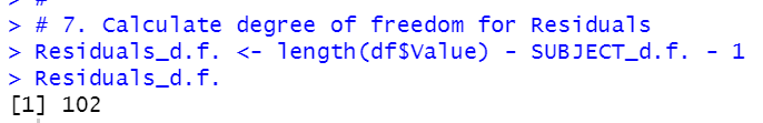
f:id:cross_hyou:20210522090108p:plain

We got 102

f:id:cross_hyou:20210522090222p:plain

Now, we got 2, 102, 779.9 and 10990.3.

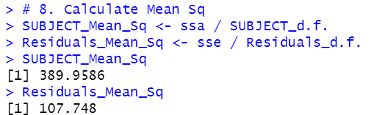
8. we can calculate Mean Sq.

SUBJECT Mean Sq = 779.9 / 2 = 389.96

Residuals Mean Sq = 10990.3 / 102 = 107.75

f:id:cross_hyou:20210522090814p:plain

f:id:cross_hyou:20210522090903p:plain


9. Calculate F-value.
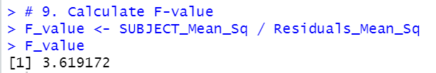
f:id:cross_hyou:20210522091115p:plain

We got 3.6192

f:id:cross_hyou:20210522091215p:plain

10. Calculate p-value

f:id:cross_hyou:20210522091709p:plain

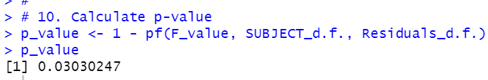
Nice! Finally we got 0.0303!

f:id:cross_hyou:20210522091853p:plain

That's it.

Next blog is...


www.crosshyou.info


If you would like to see the first blog.
 

www.crosshyou.info


OECD Threatened species data analysis 2 - visualize data using ggplot2 in R


www.crosshyou.info

 This brlog is following of above blog.
This time, let's visualize data with ggplot2 package in R.

Boxplot by SUBJECT

f:id:cross_hyou:20210517193142p:plain

f:id:cross_hyou:20210517193154p:plain

We see BIRD are the highest median and PLANT is the lowest median.


f:id:cross_hyou:20210517193322p:plain

f:id:cross_hyou:20210517193335p:plain

Next, let's visualize by LOCATION

f:id:cross_hyou:20210517194505p:plain

f:id:cross_hyou:20210517194524p:plain

CZE has the higest threatened species proportion. COL has the lowest.

That's it.

Next blog is


www.crosshyou.info


To read the 1st blog,


www.crosshyou.info