OECD Household disposable income data analysis 6 - Time-Series Data Regression using R

 Photo by Jeremy Bishop on Unsplash  

www.crosshyou.info

This post is following of above post.
In this post, I will do time-series data regression using R.

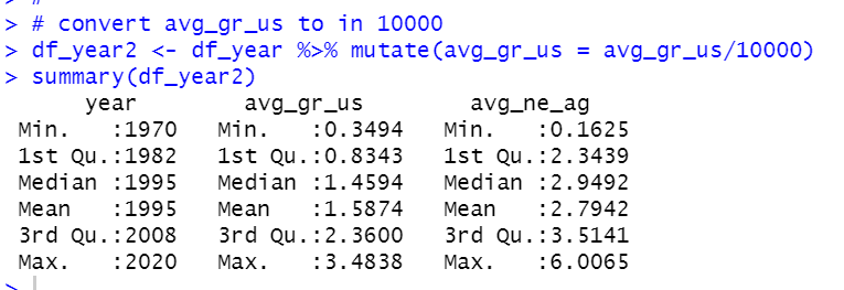
Firstly, I converted avg_gr_us in 10000 value.

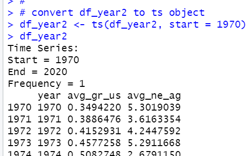
Then, I converted df_year2 data frame to ts object.

Then, I load dynlm package.

Let's begin with "static model"

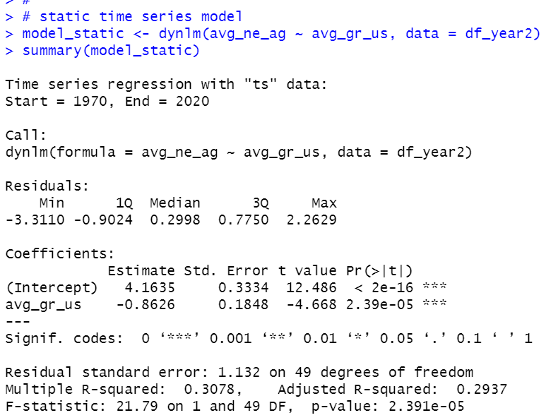
We see avg_gr_us and avg_ne_ag are negative correlation.

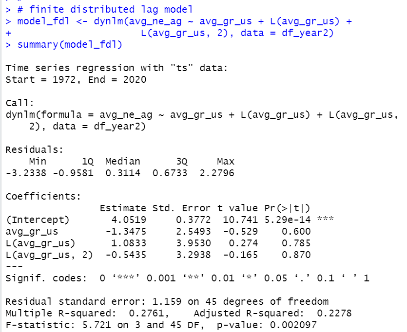
Aggregate coefficeitns are -1.3475 + 1.0833 - 0.5435 = -0.8077.

Next, load car package.

Then, I do F test to test H0: all "avg_gr_us" coefficients are = 0

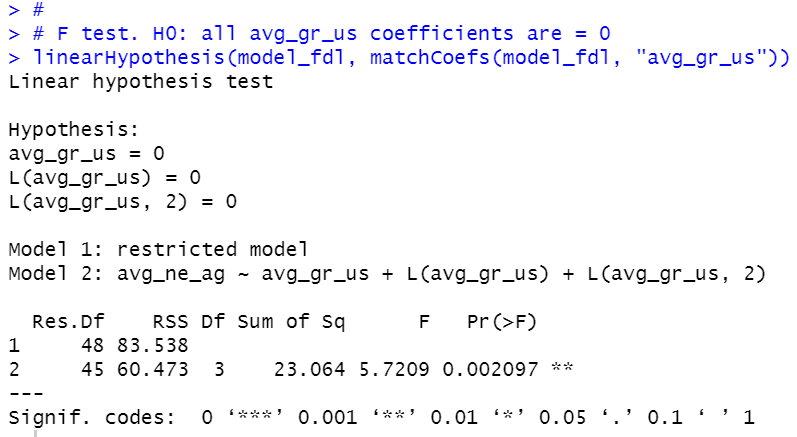
p-value is 0.002097, so I reject H0.

Then, I made trend only model.

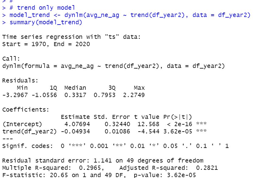
We see trend coefficient is statistically significant.

Then, I made trend + avg_gr_us model.

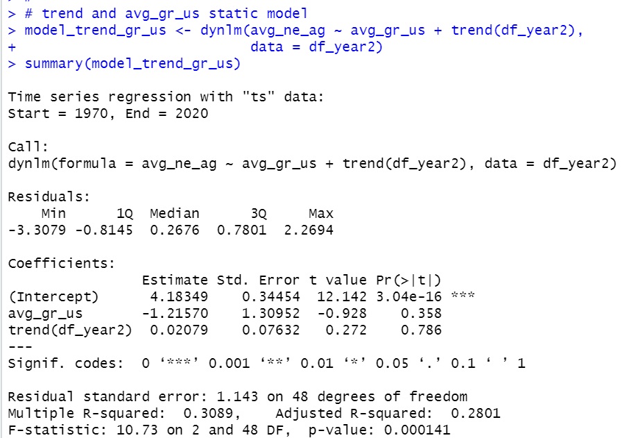
p-value is 0.000141 so this model is statistically significant.

That}s it. Thank you!

Next post is

www.crosshyou.info

To read the 1st post,

www.crosshyou.info