OECD Gender wage gap data analysis 1 - Load CSV file data into R

Photo by Trevor McKinnon on Unsplash

In this post, I will analyze OECD Gender wage gap data.

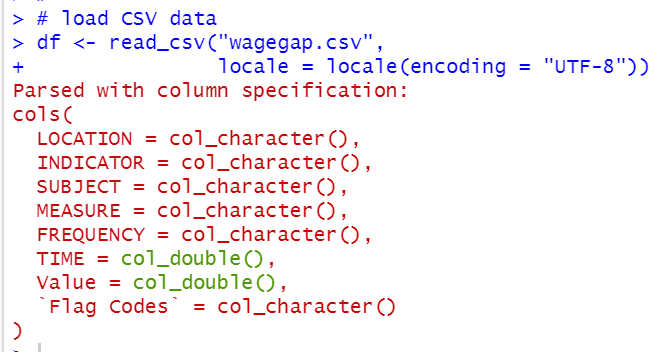
From the OECD web site, I downloaded the CSV data file like below.

I will use R to analyze this data.

First, I load tidyverse packages

Then, I use read_csv() function to load CDV data into R.

Let's check each variables.

First, LOCATION

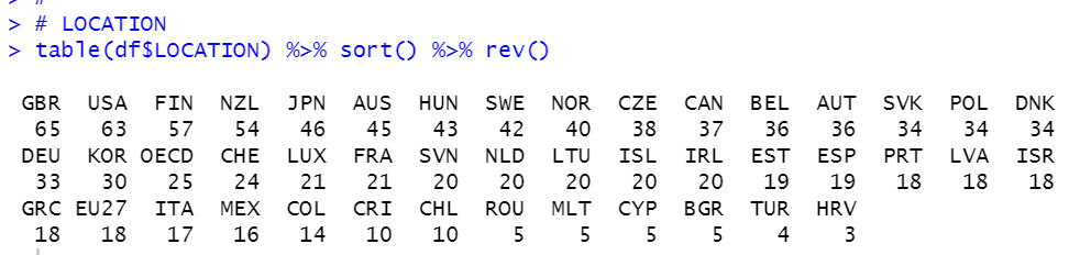
There are many locations, GBR has the most observations, 65. HRV has the least observations, 3.

INDICATOR

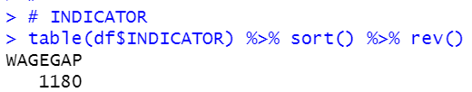
INDICATORS ha only one value, WAGEGAP. so I drop this variable from df.

SUBJECT

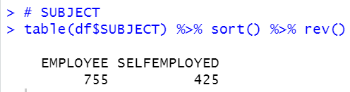
For SUBJECT, there are two subjects, one is employee and the other is selfemployed.

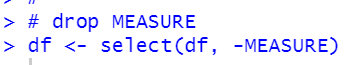
MEASURE,

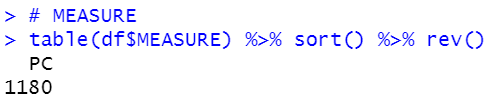
There is only one value in MEASURE, so I will drop MEASURE.

FREQUENCY

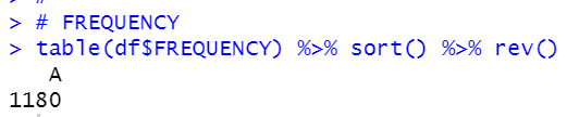
There is only one value:A in FREQUENCY, so I will drop FREQUENCY from df.

TIME

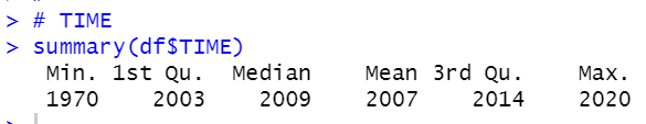
TIME is numerical data. The minimum is 1970, the maximum is 2020. Mean is 2007.
There is no NA.

Value

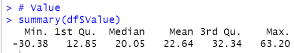
Value is numerical data. There is no NA. The minimum is -30.38, The maximum is 63.20.

Flag Codes

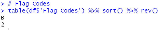
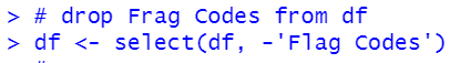
Flag Codes has only one value, B. So I will drop it.

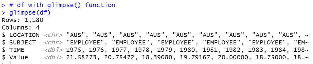
All right, let's see df with glimpse() function.

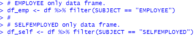
Now, we know there are EMPLOYEE and SELFEMPLOYED in subject.

Let's make two subset data frame, one is for EMPLOYEE only and the other is SELFENPLOYED only.

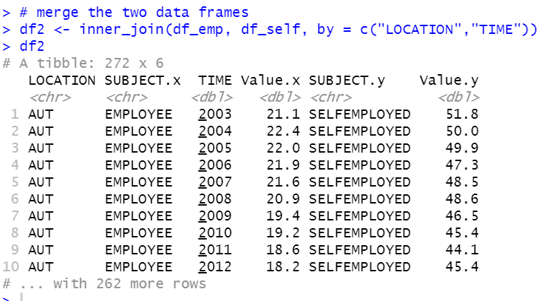
Let's merge these two data fram with inner_join() function.

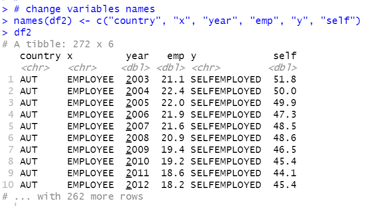
Let's change Value.x to emp, Value.y to self. Also, let's change other variables, LOCATION to country, SUBJECT.X to x, TIME to year, SUBJECT.y to y.

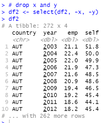
I will drop x and y.

Let's change country to factor type.

All right.
Let's see summary of df2.

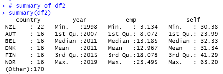
We see NZL has the most observations. year starts from 1998 to 2019. The minimum emp is -3.13 and the maximum emp us 23.5. The minimum self is -30.38 and the maximum self is 63.20.

That's it. Thank you!

Next post is...

www.crosshyou.info